The Process of Developing Species Distribution Modeling Using Maxent

Methodology

Species distribution modeling (SDM) is used to predict where a species could occur. SDM can be used to visually represent the fundamental niche of a species. This is different from the realized niche which describes where a species currently occurs. SDM uses various types of environmental data and species occurrence data to extrapolate the distribution of a species using a statistical model (Franklin 2010).

An example of the competed SDM model for Butomus umbellatus (flowing rush) can be seen below.

Software

This project utilized an open source SDM software called Maxent. Maxent generates a model by applying maximum entropy modeling which is a generalized machine learning technique. The program uses environmental data and species presence data and applies a probability distribution for each grid cell on a raster.

Data Collection

Environmental data sets used for the SDM models include WorldClim bioclimatic variables (version 2.1) and WorldClim elevation data (version 2) resulting in 20 different environmental data sets. WorldClim bioclimatic data set uses climate data from 1970 to 2000 for variable development. Both data sets are 1 Km 2 resolution.

Presence-only observational data from Washington State for each species of interest was utilized in the SDM models. Presence data was collected into a single database using the Global Biodiversity Information Facility (GBIF) looking at all target species. GBIF is an online open access network that collects data on species occurrence. Data is submitted to GBIF from governments, researchers, organizations, museums, and online crowdsourced applications around the world.

Model Building

Maxent utilized species presence data and environmental data with maximum entropy modeling to create a species distribution model (Figure 1). The initial data for each species were processed by Maxent with all 20 environmental data sets. Each species model was then evaluated to determine the highest performing variables by largest percent contribution. Only the three best performing variables were selected for the final model. The selected three variables can be seen in tables 4 and 5.

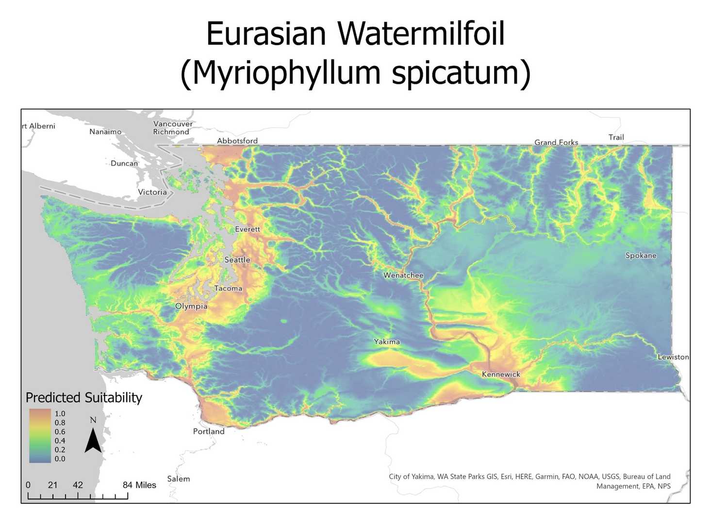
A second pass of Maxent was then used to produce the final species models utilizing only the selected environmental variables. Output models from maxent were transposed over a Washington state base map using ArcPro Regions of low (blue) and high (red) suitability for each species of interest as can be seen below.

Model Evaluation

The performance of the species models was evaluated by applying a cumulative threshold. The cumulative threshold is a chosen threshold for which a species occurrence is considered a presence or absence. Currently there is no standardized rule for setting a threshold and thus it must be chosen by the researcher (Philips et al. 2006). Fixed cumulative thresholds of 1 and 5 for evaluation have been predominantly used in literature of species distribution models (Manel et al. 1999, Bailey et al. 2002, Phillips et al. 2006). However, the use of fixed cumulative thresholds has been shown to result in more false positives and negatives (cummings 2000, Liu et al. 2005). Researchers are currently evaluating Maxent to better understand the effectiveness of using different thresholds for predictive evaluations. Due to the limited rules, the sensitivity-specificity sum maximization (SSSM) approach for the threshold was utilized. The SSSM approach produces a threshold in Maxent that results in a better threshold for evaluating models than fixed thresholds (Manuel et al. 2001, Liu et al. 2005). Sensitivity is the measure that the test was able to correctly classify where a species does occur, and specificity is the measure that a test was able to classify where a species does not occur (Parikh et al. 2008). The SSSM allows the threshold to be determined by maximizing the sum of sensitive and specificity. This is equivalent to finding a point on the receiver operating characteristic (ROC) curve whose tangent slope is equal to 1 (Cantor et al. 1999). Once the cumulative threshold is chosen, it is used to produce the extrinsic omission rate (EOR), proportional predicted area (PPA), and p-value for a model. The EOR is the fraction of test locations which are predicted as not suitable for the species. The PPA is the fraction of pixels which are predicted as suitable for the given species. The p-value represents the null hypothesis, which states that the model performs randomly (Phillips et al. 2006). A low p-value corresponds to a non-random model. A one-tailed binomial test is applied to determine if the p-value is sufficient to disprove the null hypothesis. Lower EOR rates are needed for good model predictability (Anderson et al. 2002). Large PPA values may improve quality of species potential distribution models (Phillips et al. 2006).

This project looked at the very basic process of developing SDM. This process can be further developed to refine and improve the accuracy of the results. I intend to further develop these models in the future and when I do I will post updates.

The entire paper can be downloaded from the Oregon State University's Scholars Archive.

Resources:

Bailey, S.‐A., Haines‐Young, R. H. and Watkins, C.. 2002. Species presence in fragmented landscapes: modeling of species requirements at the national level. Biol. Conserv. 108: 307–316.

Cantor, S. B. et al. 1999. A comparison of C/B ratios from studies using receiver operating characteristic curve analysis. J. Clin. Epidemiol. 52: 885– 892.

Franklin, J. (2010). Mapping Species Distributions Spatial Inference and Prediction. Cambridge University Press.

Fick, S.E. and R.J. Hijmans, 2017. WorldClim 2: new 1km spatial resolution climate surfaces for global land areas. International Journal of Climatology 37 (12): 4302-4315.

Parikh R, Mathai A, Parikh S, Chandra Sekhar G, Thomas R. Understanding and using sensitivity, specificity and predictive values. Indian J Ophthalmol. 2008 Jan-Feb;56(1):45-50. doi: 10.4103/0301-4738.37595. PMID: 18158403; PMCID: PMC2636062.

Phillips, S. J., Anderson, R. P., & Schapire, R. E. (2006). Maximum entropy modeling of species geographic distributions. Ecological Modelling, 190(3-4), 231-259. doi:10.1016/j.ecolmodel.2005.03.026

Manel, S., Williams, H. C. and Ormerod, S. J.. 2001. Evaluating presence‐absence models in ecology: the need to account for prevalence. J. Appl. Ecol. 38: 921–931.DOI: 10.1046/j.1365-2664.2001.00647.x

Liu, C., Berry, P.M., Dawson, T.P. and Pearson, R.G. (2005), Selecting thresholds of occurrence in the prediction of species distributions. Ecography, 28: 385-393. https://doi.org/10.1111/j.0906-7590.2005.03957.x